The deletion of a data item from a data structure has always been difficult whatever data structure we use. The deletion is the inverse of insertion. In deletion there is a given value x and an AVL tree T. We delete the node containing the value x and rebalance the tree if it becomes unbalance after deleting the node. We will see that the deletion of a node is considerably more complex than the insertion of a node. It is complex in the sense that we may have to do more than one rotations to rebalance the tree after deleting a node. We will discuss the deletion case by case and will see that about what points we have to take care in the deletion process.
We are not going to write the code for deletion here. If we have to use AVL tree routines or class, the deletion and insertion routines of AVL tree are available in standard library. We can use these routines in our program. We have no need to write these routines. But here we discuss these to understand their functionality.
We know that insertion in a height-balanced tree requires at most one single rotation or one double rotation. We do this rotation at the node whose balance violates the AVL condition. We can use rotations to restore the balance when we do a deletion. If the tree becomes unbalance after deleting a node then we use rotations to rebalance it. We may have to do a rotation at every level of the tree. Thus in the worst case of deletion we have to do log2 N rotations. As log2 N is the number of levels of a tree of N nodes.
Let’s consider an example of deleting a node from a tree. In this example, we will discuss the worst case of deletion that is we have to do rotation at each level after deleting a node. Look at the following figure i.e. Fig 23.8. In this figure the root of the tree is node N and we have expanded only the left subtree of this node. The right subtree of it is indicated by a triangle. We focus on the left subtree of N. The balance of each non-leaf node of the left subtree of N is –1. This means that at every non-leaf node the depth/height of left subtree is one shorter than the height of right subtree. For example look at the node C. The left subtree of C is one level deep where as it’s right subtree is two levels deep. So balance of it is 1 – 2 = -1. If we look at node I its left subtree has height 2 as there are two levels where nodes G and H exists. The right subtree of I has number of levels (i.e. height) 3 where exists the nodes K, L and M respectively. Thus the balance of I is 2 – 3 = -1. Similarly we can see that other nodes also have the balance –1. This tree is shown in the following figure.
Here in this tree, the deletion of node A from the left subtree causes the worst case of deletion in the sense that we have to do a large number of rotations. Now we delete the node A from the tree. The effect of this deletion is that if we consider the node C the height of its left subtree is zero now. The height of the right subtree of C is 2. Thus the balance of C is 2 now. This makes the tree unbalance. Now we will do a rotation to make the tree balanced. We rotate the right subtree of C that means the link between C and D so that D comes up and C goes down. This is mentioned in the figure below.
After this rotation the tree has transformed into the following figure. Now D becomes the left child of F and C becomes the left child of D.
By looking at the inorder traversal of the tree, we notice that it is preserved. The inorder traversal of the tree before rotation (i.e. fig 23.8) is C D E F G H I J K L M N. Now if we traverse the tree after rotation (i.e. fig 23.9) by inorder traversal we get C D E F G H I J K L M N, which is the same as it was before rotation.
After this rotation we see that the tree having D as root is balanced. But if we see the node F we notice that the height of its left subtree is 2 and height of its right subtree is 4. Thus the balance of F is –2 (or 2 if we take the absolute value) now. Thus the tree becomes unbalance. So we have to do rotation again to balance the tree. The whole left subtree of F is shorter so we do the left rotation on the link of F and I (in the tree in fig 23.9) to bring F down and I up so that the difference of height could be less. After rotation the tree gets the new form that is shown in the figure below.
Here we see that the nodes G and H, which were in the left subtree of I, now become the right subtree of F. We see that the tree with I as root is balanced now. Now we consider the node N. We have not expanded the right subtree of N. Although we have not shown but there may be nodes in the right subtree of N. If the difference of heights of left and right subtree of N is greater than 1 then we have to do rotation on N node to balance the tree.
Thus we see that there may be such a tree that if we delete a node from it we have to do rotation at each level of the tree. We notice that we have to do more rotations in deletion as compared to insertion. In deletion when we delete a node we have to check the balance at each level up to the root. We do rotation if any node at any level violates the AVL condition. If nodes at a level do not violate AVL condition then we do not stop here we check the nodes at each level and go up to the root. We know that a binary tree has log2 N levels (where N is total number of nodes) thus we have to do log2 N rotations. We have to identify the required rotations that mean we have to identify that which one rotation out of the four rotations (i.e. single left rotation, single right rotation, double right-left rotation and double left-right rotation) we have to do. We have to identify this at each level.
We can summarize the deletion procedure as under.
Delete the node as in binary search tree. We have seen in the discussion of deleting a node from a BST that we have three cases, which we discussed as follows
Case I: The node to be deleted is the leaf node i.e. it has no right or left child. It is very simple to delete such node. We make the pointer in the parent node pointing to this node as NULL. If the memory for the node has been dynamically allocated, we will release it.
Case II: The node to be deleted has either left child (subtree) or right child (subtree).
In this case we bypass the node in such a way that we find the inorder successor of this node and then link the parent of the node to be deleted to this successor node. Thus the node was deleted.
Case III: The node to be deleted has both the left and right children (subtree). This is the most difficult case. In this case we find the inorder successor of the node. The left most node of the right subtree will be the inorder successor of it. We put the value of that inorder successor node into the node to be deleted. After it we delete the inorder successor node recursively.
In deletion in AVL tree, we delete the node as we delete it in a BST. In third case of deletion in BST we note that the node deleted will be either a leaf or have just one subtree (that will be the right subtree as node deleted is the left most subtree so it cannot have a left subtree). Now we are talking about deletion in an AVL tree. Since this is an AVL tree so if the deleted node has one subtree that subtree contains only one node. Why it is so? Think about its reason and answer.
After deleting the node we traverse up the tree from the deleted node checking the balance of each node at each level up to the root. Thus the deletion in AVL tree is like the deletion in BST except that here in AVL tree we have to rebalance the tree using rotations.
Cases of Deletion in AVL Tree
Now let’s consider the cases of deletion that will help to identify what rotation will be applied at what point.
There are 5 cases to consider. Let’s go through the cases graphically and determine what actions are needed to be taken. We will not develop the C++ code for deleteNode in AVL tree. This is left as an exercise.
Case 1a:
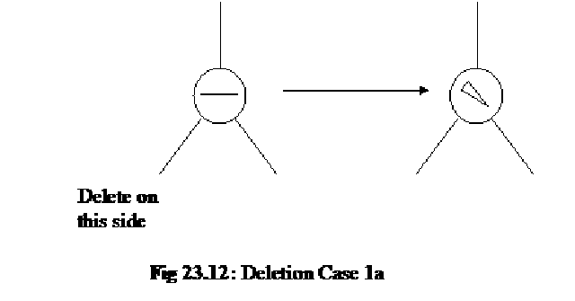
The first case is that the parent of the deleted node had a balance of 0 and the node was deleted in the parent’s left subtree.
In the following figure (Fig 23.12) the left portion shows the parent node with a horizontal line in it. This horizontal line indicates that the left and right subtrees of this node have the same heights and thus the balance of this node is 0. When we delete a node from its left subtree then height of its right subtree becomes larger than the left subtree. The right portion in the figure shows this. We are showing a symbol instead of balance of node inside the node. The notation (symbol) in the node indicates that the height of left subtree is shorter than the height of right subtree of the node.
Now the action that will be taken in this case is that, change the balance of the parent node and stop. No further effect on balance of any higher node. There is no need of rotation in this case. Thus it is the easiest case of deletion.
Let’s consider an example to demonstrate the above case.
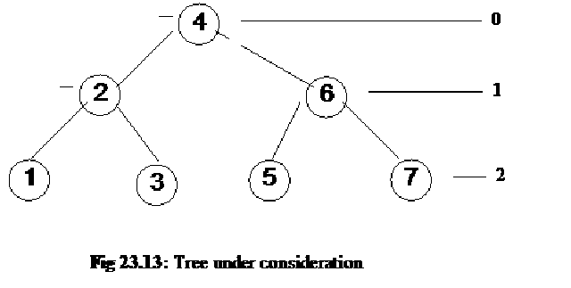
Consider the tree shown in the following figure i.e. Fig 23.13. This is a perfectly balanced tree. The root of this tree is 4 and nodes 1, 2 and 3 are in its left subtree. The nodes 5, 6 and 7 are in the right subtree.
Consider the node 2. We have shown the balance of this node with a horizontal line, which indicates that the height of its left subtree is equal to that of its right subtree. Similarly we have shown the balance of node 4.
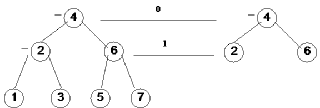
Now we remove the node 1 which is the left subtree of node 2. After removing the left child (subtree) of 2 the height of left subtree of 2 is 0. The height of right subtree of 2 is 1 so the balance of node 2 becomes –1. This is shown in the figure by placing a sign that is down ward to right side, which indicates that height of right subtree is greater than left subtree. Now we check the node 4. Here the height of left subtree of it is still 2. The height of its right subtree is also 2. So balance of the node 4 is 0 that is indicated by the small horizontal line (minus sign) in the figure below. Here we don’t need to change the balance of 4.
    
| | | | | | | |
| |  | |  |
| | | |  |
|
|
|
|
| Fig 23.14: Tree before and after deleting node 1 |
|
|
Case 1b:
This case is symmetric to case 1a. In this case, the parent of the deleted node had a balance of 0 and the node was deleted in the parent’s right subtree. The following figure shows that the balance of the node was zero as left and right subtree of it have the same heights.
After removing the right child the balance of it changes and it becomes 1, as the height of its left subtree is 1 greater than the height of right subtree. The action performed in this case is the same as that in case 1a. That is change the balance of the parent node and stop. No further effect on balance of any higher node.
The previous example can be done for this case only with the change that remove the right child of node 2 i.e. 3.
Case 2a:
This is the case where the parent of the deleted node had a balance of 1 and the node was deleted in the parent’s left subtree. This means that the height of left subtree of the parent node is 1 greater than the height of its right subtree. It is shown in the left portion of the figure below.
Now if we remove a node from the left subtree of this node then the height of left subtree will decrease by 1 and get equal to the height of right subtree. Thus the balance of this node will be zero. In this case, the action that we will perform to balance the tree is that change the balance of the parent node. This deletion of node may have caused imbalance in higher nodes. So it is advised to continue up to the root of the tree. We will do rotation wherever the balance of the node violates the AVL condition.
There are five cases to consider while deleting a node of an AVL tree. When a node is deleted, the tree can become unbalanced. We calculate the balance factor of each node and perform rotation for unbalanced nodes. But this rotation can prolong to the root node. In case of insertion, only one node’s balance was adjusted as we saw in previous lectures but in case of deletion, this process of rotation may expand to the root node. However, there may also be cases when we delete a node and perform no or one rotation only.
Now, we will see the five cases of deletion. A side note is that we are not going to implement these cases in C++ in this lecture, you can do it yourself as an exercise with the help of the code given inside your text book. In this lecture, the emphasis will be on the deletion process and what necessary actions we take when a node is required to be deleted from an AVL tree. Actually, there are two kinds of actions taken here, one is deletion and the other one is the rotation of the nodes.
Case 1a: The parent of the deleted node had a balance of 0 and a node was deleted in the parent’s left subtree.
In the left tree in the Fig 24.1, the horizontal line inside the tree node indicates that the balance is 0, the right and left subtrees of the node are of equal levels. Now, when a node is deleted from the left subtree of this node, this may reduce by one level and cause the balance of the right subtree of the node to increase by 1 relatively. The balance of the node in favor of the right subtree is shown by a triangular knob tilted towards right. Now, the action required in this case to make the tree balanced again is:
Change the balance of the parent node and stop. There is no further effect on balance of any higher node.
In this case, the balance of the tree is changed from 0 to –1, which is within the defined limits of AVL tree, therefore, no rotation is performed in this case.
Below is a tree in which the height of the left subtree does not change after deleting one node from it.
The node 4 is the root node, nodes 2 and 6 are on level 1 and nodes 1, 3, 5, 7 are shown on level 2. Now, if we delete the node 1, the balance of the node 2 is tilted towards right, it is –1. The balance of the root node 4 is unchanged as there is no change in the number of levels within right and left subtrees of it. Similarly, there is no change in the balances of other nodes. So we don’t need to perform any rotation operation in this case.
Let’s see the second case.
Case 1b: the parent of the deleted node had a balance of 0 and the node was deleted in the parent’s right subtree.
On the left of Fig 24.3, the tree is within the balance limits of AVL. After a node is deleted from the right subtree of it. The balance of the tree is tilted towards left as shown in the right tree show in the Fig 24.3. Now, we see what action will be required to make the tree balanced again.
Change the balance of the parent node and stop. No further effect on balance of any higher node (same as 1a).
So in this case also, we don’t need to perform rotation as the tree is still an AVL (as we saw in the Case 1a). It is important to note that in both of the cases above, the balance of the parent node was 0. Now, we will see the cases when the balance of the parent node is not 0 previously.
Case 2a: The parent of the deleted node had a balance of 1 and the node was deleted in the parent’s left subtree.
In the Fig 24.4 above, the tree on the left contains the balance factor as 1, which means that the left subtree of the parent node is one level more than the number of levels in the right subtree of it. When we delete one node from the left subtree of the node, the height of the left subtree is changed and the balance becomes 0 as shown in the right side tree of Fig 24.4. But it is very important understand that this change of levels may cause the change of balance of higher nodes in the tree i.e.
Change the balance of the parent node. May have caused imbalance in higher nodes so continue up the tree.
So in order to ensure that the upper nodes are balanced, we calculate their balance factors for all nodes in higher levels and rotate them when required.
Case 2b: The parent of the deleted node had a balance of -1 and the node was deleted in the parent’s right subtree.
Similar to the Case 2a, we will do the following action:
Change the balance of the parent node. May have caused imbalance in higher nodes so continue up the tree.
Now, we see another case.
Case 3a:The parent had balance of -1 and the node was deleted in the parent’s left subtree, right subtree was balanced.
As shown in the left tree in Fig 24.5, the node A is tilted towards right but the right subtree of A (node B above) is balanced. The deleted node lies in the left subtree of the node A. After deletion, the height of the left subtree is changed to h-1 as depicted in the right tree of above figure. In this situation, we will do the following action:
Perform single rotation, adjust balance. No effect on balance of higher nodes so stop here.
After single left rotation, we have the tree as shown in the figure below.
Node A has become the left subtree of node B and node 2 left subtree of node B has become the right subtree of node A. The balance of node B is tiled towards left and balance of node A is tilted towards right but somehow, both are within AVL limits. Hence, after a single rotation, the balance of the tree is restored in this case.
Case 4a: Parent had balance of -1 and the node was deleted in the parent’s left subtree, right subtree was unbalanced.
In the last case 3a, the right subtree of node A was balanced. But in this case, as shown in the figure above, the node C is tilted towards left. The node to be deleted lies in the left subtree of node A. After deleting the node the height of the left subtree of node A has become h-1. The balance of the node A is shown tilted towards right by showing two triangular knobs inside node A. So what is the action here.
Double rotation at B. May have affected the balance of higher nodes, so continue up the tree.
By performing double rotation in the tree above, we have the following tree.
Node A, which was the root node previously, has become the left child of the new root node B. Node C, which was the right child of the root node C has now become the right child of the new root node B.
Case 5a: The parent had balance of -1 and the node was deleted in the parent’s left subtree, right subtree was unbalanced.
In the figure above, the right tree of the node B has a height of h-1 while the right subtree is of height h. When we remove a node from the left subtree of node A, the new tree is shown on the right side of Fig 24.9. The subtree 1 has height h-1 now, while subtrees 2 and 3 have the same heights. So the action we will do in this case is:
Single rotation at B. May have effected the balance of higher nodes, so continue up the tree.
These were the five cases of deletion of a node from an AVL tree. Until now, we are trying to understand the concept using the figures. You might have noticed the phrase ‘continue up the tree’ in the actions above. How will we do it? One way is to maintain the pointer of the parent node inside each node. But often the easiest method when we go in downward direction and then upward is recursion. In recursion, the work to be done later is pushed on to the stack and we keep on moving forward until at a certain point we back track and do remaining work present in the stack. We delete a node when we reach at the desired location and then while traversing back, do the rotation operation on our way to the root node.
Symmetrical to case 2b, we may also have cases 3b, 4b and 5b. This should not be a problem in doing it yourself.
Other Uses of Binary Trees
A characteristic of binary trees is that the values inside nodes on the left of a node are smaller than the value in the node. And the values inside the nodes on the right of a node are greater than the value in the node. This is the way a binary tree is constructed.
Whatever is the size of the tree, the search is performed after traversing upto log2n levels maximum.
We have observed that the binary tree becomes a linked list and it can become shallow. The AVL conditions came into picture to control the height balance of a binary tree. While searching in an AVL tree, in the worst case scenario we have to search 1.44 log2n levels. For searches, binary and AVL trees are the most efficient but we do have some other kinds of trees that will be studied later.
Lets see what could be some other uses of binary trees, we start our discussion with Expression Trees.
Expression Trees
Expression trees, the more general parse trees and abstract syntax trees are significant components of compilers.
We already know about compilers that whenever we write our program or code in some computer language like C++ or Java. These programs are compiled into assembly language or byte code (in case of Java). This assembly language code is translated converted into machine language and an executable file is made by another program called the assembler.
By the way, if you have seen your syllabus, you might have seen that there is a dedicated subject on compilers. We study in detail about compilers in that course. For this course, we will see expression or parse trees.
We will take some examples of expression trees and we will not delve into much depth of it rather that would be an introduction to expression trees.
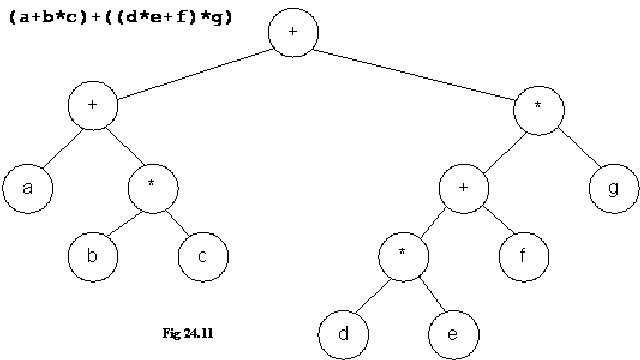
You can see the infix expression above (a + b * c) + ( (d * e + f) * g), it is represented in the tree form also.
You can see from bottom of the tree that the nodes b and c in the nodes are present at the same level and their parent node is multiplication (*) symbol. From the expression also, we see that the b and c are being multiplied. The parent node of a is + and right subtree of + is b*c. You might have understood already that this subtree is depicting a+b*c. On the right side, node d and e are connected to the parent *. Symbol + is the parent of * and node f. The expression of the subtree at node + is d*e+f. The parent of node + is * node, its right subtree is g. So expression of the subtree at this node * is (d*e+f)*g). The root node of the tree is +.
These expression trees are useful in compilers and in spreadsheets also, they are sometimes called parse trees.
Parse Tree in Compilers
See the expression tree of expression A := A + B * C below. We are adding B and C, adding the resultant in A and then finally assigning the resultant to A.
The root node in the parse tree shown above is <assign>.
The assignment statement (<assign>) has three parts. On the left of it, there is always an identifier (single or an array reference) called l-value. The l-value shown in the tree above is <id> and the identifier is A in the expression above. The second part of assignment statement is assignment operator (= or :=). One the right of assignment operator lies the third part of assignment statement, which is an expression. In the expression A := A + B * C above , the expression after assignment operator is A + B * C. In the tree, it is represented by the node <expr>. The node <expr> has three subnodes: <expr>, + and <term>. <expr>’s further left subtree is <expr>, <term>, <factor>, <id> and then finally is B. The right subchild <term> has further subnodes as <term>, * and <factor>. <factor> has <id> as subchild and <id> has C.
Note the nodes in gray shade in the tree above form A = A + B * C.
Compiler creates these parse trees. We will see how to make these trees, when we will parse any language tree like C++. Parsing mean to read and then extract the required structure. A compiler parses a computer language like C++ to form parse trees. Similarly, when we do speech recognition. Each sentence is broken down into a certain structure in form of a tree. Hand writing recognition also involves this. The tablet PCs these days has lot of implementation of parse trees.
Parse Tree for an SQL Query
Let’s see another example of parse trees inside databases. The parse trees are used in query processing. The queries are questions to the databases to see a particular kind of data. Consider you have a database for a video store that contains data of movies and artists etc. You are querying that database to find the titles of movies with stars born in 1960. The language used to query from the database is called SQL (Structured Query Language), this language will be dealt in depth in the databases course. The tables lying in this movies database are:
StarsIn(title, year, starName)
MovieStar(name, address, gender, birthdate)
The following SQL query is used to retrieve information from this database:
SELECT title
FROM StarsIn, MovieStar
WHERE starName = name AND birthdate LIKE ‘%1960’ ;
This query is asking to retrieve the titles of those movies from StarsIn and MovieStar tables where the birthdate of an actor is 1960. We see in query processing a tree is formed as shown in the figure below:
The root node is Query. This node is further divided into SELECT, <SelList>, FROM, <FromList>, WHERE and <Condition> subnodes. <SelList> will be an Attribute and finally a title is reached. Observe the tree figure above, how the tree is expanded when we go in the downward direction. When the database engine does the query process, it makes these trees. The database engine also performs query optimization using these trees.
Compiler Optmization
Let’s see another expression tree here:
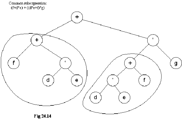
The root node is +, left subtree is capturing the f+d*e expression while the right subtree is capturing (d*e+f)*g.
Normally compilers has intelligence to look at the common parts inside parse trees. For example in the tree above, the expressions f+d*e and d*e+f are same basically. These common subtrees are called common subexpressions. To gain efficiency, instead of calculating the common subexpressions again, the compilers calculates them once and use them at other places. The part of the compiler that is responsible to do this kind of optimization is called optimizer.
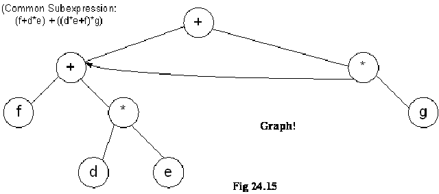
See the figure below, the optimizer (part of compiler) will create the following graph while performing the optimization. Because both subtrees were equivalent, it has taken out one subtree and connected the link from node * to node +.
This figure is not a tree now because it has two or more different paths to reach a node. Therefore, this has become a graph. The new connection is containing a directed edge, which is there in graphs.
Optimizer uses the expressions trees and converts them to graphs for efficiency purposes. You read out from your book, how the expression trees are formed, what are the different methods of creating them.
Technorati Tags:
ds tutorial,
data structure tutorial,
tree data structure,
trees in data structure,
tree ds,
tree traversal data structure,
tree types,
types of trees,
binary trees,
binary search trees,
bst,
bst data structure,
bst ds,
complete binary search tree,
non tree structure,
linear tree,
avl tree,
avl tree traversal,
avl data structure,
avl ds,
avl tree rotation,
rotation of avl tree,
avl tree tutorial,
expression trees


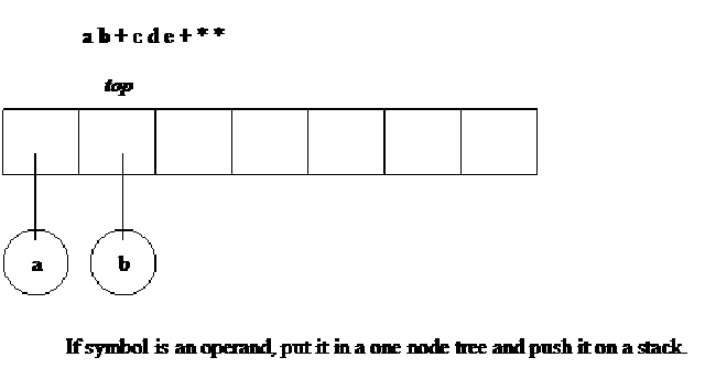
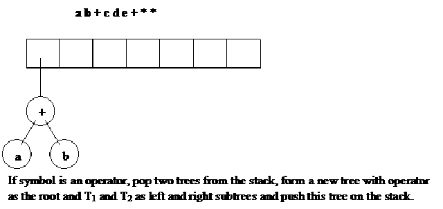
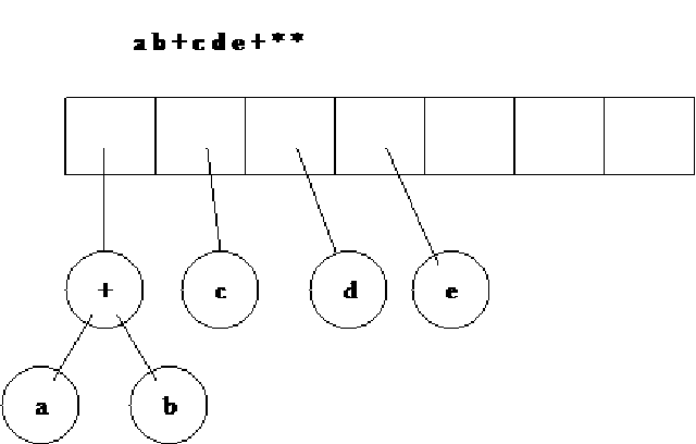




![clip_image001[4] clip_image001[4]](http://lh5.ggpht.com/-tKOX_k34JOc/UKkxiBunT7I/AAAAAAAABzc/6Ngm56623-E/clip_image0014_thumb%25255B1%25255D.gif?imgmax=800)
![clip_image003[4] clip_image003[4]](http://lh5.ggpht.com/-o_gBDa_Uqok/UKkxlg7B8dI/AAAAAAAABzs/XhLiJBq5-gs/clip_image0034_thumb%25255B1%25255D.gif?imgmax=800)
![clip_image004[4] clip_image004[4]](http://lh3.ggpht.com/-qqV3FyUBoN0/UKkxoNMJyBI/AAAAAAAABz8/zUMUGkm9bfE/clip_image0044_thumb%25255B1%25255D.gif?imgmax=800)
![clip_image005[4] clip_image005[4]](http://lh3.ggpht.com/-z1sQxncOFp8/UKkxqYzMcpI/AAAAAAAAB0M/oCKXtqtITX8/clip_image0054_thumb%25255B1%25255D.gif?imgmax=800)
![clip_image007[4] clip_image007[4]](http://lh5.ggpht.com/-Si3WUBgRDqo/UKkxtsoFl8I/AAAAAAAAB0c/6cCJoJ-49RA/clip_image0074_thumb%25255B1%25255D.gif?imgmax=800)
![clip_image009[4] clip_image009[4]](http://lh3.ggpht.com/-kgkwA4QiDag/UKkxwWg8IPI/AAAAAAAAB0s/jgGEZfNFBq8/clip_image0094_thumb%25255B1%25255D.gif?imgmax=800)
![clip_image011[4] clip_image011[4]](http://lh6.ggpht.com/-acoaFpISBeU/UKkxzlF2kZI/AAAAAAAAB08/408ZMtHSrhI/clip_image0114_thumb%25255B1%25255D.gif?imgmax=800)
![clip_image013[4] clip_image013[4]](http://lh3.ggpht.com/-T4ReoAceEz8/UKkx3Ok1jyI/AAAAAAAAB1M/jZCMIuIFrh4/clip_image0134_thumb%25255B1%25255D.gif?imgmax=800)
![clip_image015[4] clip_image015[4]](http://lh6.ggpht.com/-8Q5A9YwNrbg/UKkx6pdOuJI/AAAAAAAAB1c/E0kLbqpXjTU/clip_image0154_thumb%25255B1%25255D.gif?imgmax=800)
![clip_image017[10] clip_image017[10]](http://lh6.ggpht.com/-iL2GfbQKYLg/UKkx95OZwLI/AAAAAAAAB1s/my48TZnuDVE/clip_image01710_thumb%25255B1%25255D.gif?imgmax=800)


![clip_image002[5] clip_image002[5]](http://lh6.ggpht.com/-_oZBR_UgsQw/UKkuRY4XSAI/AAAAAAAABps/5ULLITn-ItI/clip_image0025_thumb1.gif?imgmax=800)

![clip_image004[5] clip_image004[5]](http://lh5.ggpht.com/-dpIhHI6Rtls/UKkuWorphEI/AAAAAAAABqM/X_rB7qoT-u4/clip_image0045_thumb1.gif?imgmax=800)
![clip_image006[5] clip_image006[5]](http://lh4.ggpht.com/-dhXCUeF9pkM/UKkub-IDz_I/AAAAAAAABqo/66r43WN6Y8M/clip_image0065_thumb1.gif?imgmax=800)


